Algorithms:
| Algorithms | Time Complexity |
|---|---|
| Euclid’s Algorithm | |
| Middle-school procedure | |
| Maximum Element | |
| Matrix Multiplication | |
| Conventional Matrix Multiplication | |
| Strassen’s Matrix Multiplication | ≈ |
| Counting binary digits | |
| Counting bits | |
| The Tower of Hanoi Puzzle | |
| String Matching | |
| Closest-Pair by Brute-force | |
| Closest-Pair by devide and conquer | |
| Convex-hull Problem by Brute-force | |
| Convex-hull Problem by devide and conquer | |
| Traveling Salesman Problem | |
| The Assignment Problem | |
| Knapsack Problem | |
| Decrease by constant factor | |
| Multiplication à la russe | |
| Exponentiation by Squaring | |
| Lumoto Partition | or |
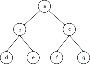
| Pre-Order | |
| In-Order | |
| Pre-Order | |
| First Multiplication of Large Integers | |
| Second Multiplication of Large Integers | |
| BFS | or |
| DFS |
| Sorting Algorithms | Best Case | Average Case | Worst Case | Stable | In-place |
|---|---|---|---|---|---|
| Selection Sort | ❌ | ✔️ | |||
| Bubble Sort | ✔️ | ✔️ | |||
| Insertion Sort | ✔️ | ✔️ | |||
| Merge Sort | ✔️ | ❌ | |||
| Quick Sort | ❌ | ✔️ | |||
| Topology Sort | — | — | |||
| Median Selection | — | — | |||
| Quick Select | — | — | |||
| Binary Search | — | — | |||
| Sequential Search | — | — |
Note:
- Topology Sort:
- If it represented by a matrix it’s complexity will be
- if it represented by a list it’s complexity will be
In The Exam Choose or
BFS & DFS Time explanation:
- BFS:
- where is the branch factor and all leaves are of depth .
- DFS:
- where is the branch factor and is maximum depth of any node.

How and are equal the first one looks like a linear complexity and second one is exponential.
In the first, the graph is the input, so it is linear in the size of the input - the graph.
The second is also linear in the size of the graph - and exponential in the depth of the solution - a different factor, still - no need to traverse a vertex more then once, so still linear in the graph’s size.
So, in here - basically is a subset of , and is more informative then it, if you can ‘suffer’ the fact that your complexity is a function of , which is not part of the input.
When we talk about big notation it means that upper bound whatsoever the input may be it should remains the same because its an upper bound. whether Big only deals with some finite data input?
Sorting key
- A specially chosen piece of information used to guide sorting. E.g., (sort student records by names.)
Two properties of sorting algorithms:
- Stability: A sorting algorithm is called stable if it preserves the relative order of any two equal elements in its input.
- In place: A sorting algorithm is in place if it does not require extra memory, except, possibly, for a few memory units.
String matching:
- searching for a given word/pattern in a text.
DEFINITION: A set of points in the plane is called convex if, for any two points and in the set, the entire line segment with the endpoints at and belongs to the set.
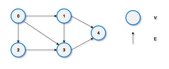
Graph:
-
A graph is a collection of points called vertices, some of which are connected by line segments called edges.
-
A graph is defined by a pair of two sets: a finite set of items called vertices and a set of vertex pairs called edges.
-
Undirected and directed graphs (digraphs).
-
What’s the maximum number of edges in an undirected graph with vertices?
-
Complete, dense, and sparse graphs
- A graph with every pair of its vertices connected by an edge is called complete,
-
Examples of Graph Algorithms:
- Graph traversal algorithms
- Shortest-path algorithms
- Topological sorting
-
Graph Representation:
- Adjacency matrix
- boolean matrix if is .
- The element on the row and column is 1 if there’s an edge from the vertex to the vertex; otherwise 0.
- The adjacency matrix of an undirected graph is symmetric.
- Adjacency linked lists
- A collection of linked lists, one for each vertex, that contain all the vertices adjacent to the list’s vertex.
- Adjacency matrix
Paths
-
A path from vertex to of a graph is defined as a sequence of adjacent (connected by an edge) vertices that starts with and ends with .
-
Simple paths: All edges of a path are distinct.
-
Path lengths: the number of edges, or the number of vertices – 1.
Connected graphs
- A graph is said to be connected if for every pair of its vertices and there is a path from to .
Connected component
- The maximum connected sub-graph of a given graph.
Cycle
- A simple path of a positive length that starts and ends at the same vertex.
Acyclic graph
- A graph without cycles
- DAG (Directed Acyclic Graph)
Cyclic graph
- A graph that contains at least one cycle
Degree of a vertex

- In-degree: In-degree of a vertex is the number of edges coming to the vertex.
- In-degree of vertex
- In-degree of vertex
- In-degree of vertex
- In-degree of vertex
- In-degree of vertex
- Out-degree: Out-degree of a vertex is the number edges which are coming out from the vertex.
- Out-degree of vertex
- Out-degree of vertex
- Out-degree of vertex
- Out-degree of vertex
- Out-degree of vertex
- The graphs are classified into various categories such as directed, non-directed, connected, non-connected, simple and multi-graph (multiple edges).
- A vertex in a graph can be connected to any number of other vertices using edges.
- An edge can be bidirected or directed.
- An edge can be weighted.
- A graph can have loops and self-loops.
Trees
- A tree (or free tree) is a connected acyclic graph.
Properties of trees:
- For every two vertices in a tree, there always exists exactly one simple path from one of these vertices to the other. Why?
- Rooted trees: The above property makes it possible to select an arbitrary vertex in a free tree and consider it as the root of the so, called rooted tree.
- =
Rooted Trees
-
Depth of a vertex
- The length of the simple path from the root to the vertex.
-
Height of a tree
- The length of the longest simple path from the root to a leaf.
Ordered trees
- An ordered tree is a rooted tree in which all the children of each vertex are ordered.
Binary trees
- A binary tree is an ordered tree in which every vertex has no more than two children, and each child is designated is either a left child or a right child of its parent.
Binary search trees
- Each vertex is assigned a number.
- A number assigned to each parental vertex is larger than all the numbers in its left subtree and smaller than all the numbers in its right subtree.
Tree search terminology
- Root : no parent.
- Leaf: no child.
- Height: distance from root to leaf (maximum Successor number of edges in path from root)
- Level (depth): number of edge in the path from the root to that node.
- Branch: Internal node, neither the root nor the leaf.
- Successor nodes of a node: its children
- Predecessor node of a node: its parent
- Path: Sequence of nodes along the edges of a tree
- Frontier: The set of all leaf nodes available for expansion at any given point (nodes in memory)
The differences between Tree and Graph
| Basis For Comparison | Tree | Graph |
|---|---|---|
| Path | Only one between two vertices | more than one path is allowed |
| Root node | It has exactly one root node | Graph doesn’t have a root node |
| Loops | no loops are permitted | Graph can have loops |
| Complexity | Less Complex | More Complex |
| Traversal technique | Pre-order, In-order, Post-order | BFS, DFS |
| Number of edges | ( is the number of node) | not defined |
| Model type | Hierarchical | Network |
Uniformed search strategies
-
The uninformed search (also called blind search or unguided search).
-
Blind search means that the strategies have no additional information about states beyond that provided in the problem definition.
-
All search strategies are distinguished by the order in which nodes are expanded.
-
Examples:
- Breadth-first search
- Uniform-cost search
- Depth-first search
- Depth-limited search
- Iterative deepening depth-
- first search
- Bidirectional search
Breadth First Search (BFS) (Shortest path first)
-
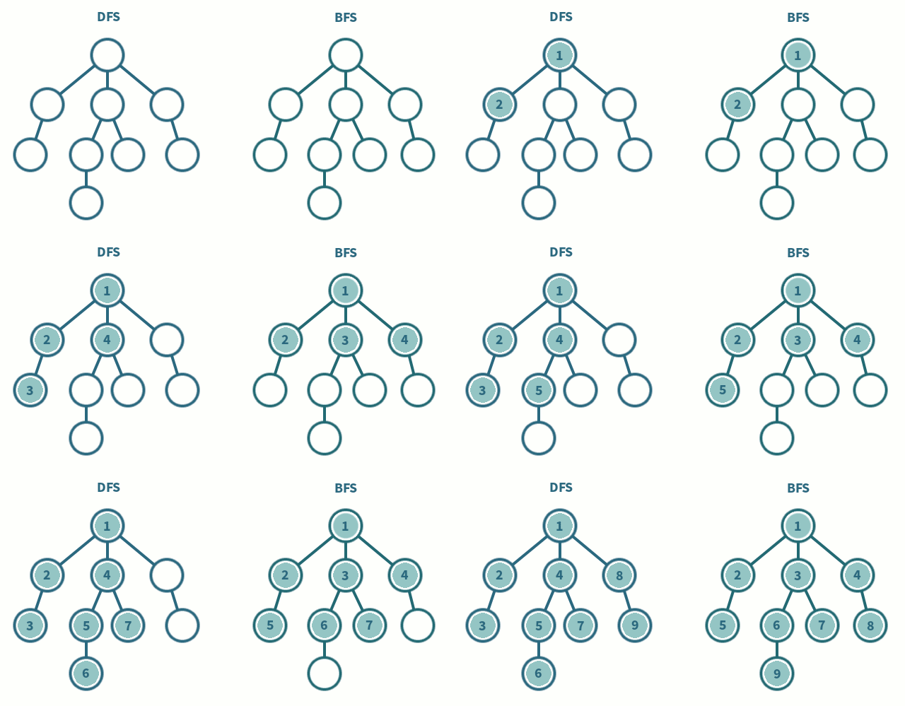
Breadth-first search is a simple strategy in which the root node is expanded first, then all the SEARCH successors of the root node are expanded next, then their successors, and so on.
-
In general, all the nodes are expanded at a given depth in the search tree before any nodes at the next level are expanded.
-
Time Complexity
- assume (worst case) that there is 1 goal leaf at the RHS so BFS will expand all nodes
- =
- =
-
Space Complexity
- how many nodes can be in the queue (worst-case)?
- at depth d there are bd unexpanded nodes in the
-
complete, optimal
Depth First Search (DFS) (Longest path first)
-
Depth-first search always expands the deepest node in the current frontier of the search tree.
-
Time Complexity
- Assume (worst case) that there is 1 goal leaf at the RHS so DFS will expand all nodes ( is maximum depth of any node)
- =
- =
-
Space Complexity
- How many nodes can be in the queue (worst-case)?
- at depth we have nodes at depth we have nodes total =
- How many nodes can be in the queue (worst-case)?
-
Infinite, not complete, not optimal
Comparing DFS and BFS:
-
Same worst-case time Complexity, but
-
In the worst-case BFS is always better than DFS
-
Sometime, on the average DFS is better if:
- many goals, no loops and no infinite paths
-
-
BFS is much worse memory-wise
-
DFS is linear space
-
BFS may store the whole search space.
-
-
In general
-
BFS is better if goal is not deep, if infinite paths, if many loops, if small search space
-
DFS is better if many goals, not many loops,
-
DFS is much better in terms of memory
-
-
Visualization of the two algorithms:

Tree Traverse:
-
Pre-Order: Process all nodes of a tree by processing the root, then recursively processing all subtrees.
-
In-Order: Process all nodes of a tree by recursively processing the left subtree, then processing the root, and finally the right subtree.
-
Post-Order: Process all nodes of a tree by recursively processing all subtrees, then finally processing the root.
Arrays
- A sequence of n items of the same data type that are stored contiguously in computer memory and made accessible by specifying a value of the array’s index.
Linked List
- A sequence of zero or more nodes, each containing two kinds of information: some data and one or more links called pointers to other nodes of the linked list.
- Singly linked list (next pointer)
- Doubly linked list (next + previous pointers)
Stacks
- A stack of plates
- insertion/deletion can be done only at the top.
- LIFO
- Two operations (push and pop)
Queues
- A queue of customers waiting for services
- Insertion/enqueue from the rear and deletion/dequeue from the front.
- FIFO
- Two operations (enqueue and dequeue)
Priority queues (implemented using heaps)
- A data structure for maintaining a set of elements, each associated with a key/priority, with the following operations:
- Finding the element with the highest priority
- Deleting the element with the highest priority
- Inserting a new element
- Scheduling jobs on a shared computer
| Comp | Array | Linked Lists |
|---|---|---|
| Length | fixed length | dynamic length |
| Memory | contiguous memory locations | arbitrary memory locations |
| Access | direct access | access by following links |
Comparing Orders of Growth (Limit)
-
:
- implies that has smaller order of growth than
- implies that has the same order of growth than
- implies that has larger order of growth than
-
=
-
Useful summation formulas and rules
-
= =
-
= =
-
= =
-
= =
-
What is Brute Force?
- A straightforward approach to solving a problem, usually based on problem statement and definitions of the concepts involved
- “Force” comes from using computer power not intellectual power
- In short, “brute force” means “Just do it!”
- Examples:
- Consecutive Integer Checking for gcd(m, n)
- Definition based matrix-multiplication
- It is the only general approach that always works
- Seldom gives efficient solution, but one can easily improve the brute force version.
- Usually can solve small sized instances of a problem
Exhaustive Search
-
Many Brute Force Algorithms use Exhaustive Search
-
A brute force solution to a problem involving search for an element with a special property, usually among combinatorial objects such as permutations, combinations, or subsets of a set.
-
Example:
- Brute force The Closest Pair
- Traveling Salesman Problem (TSP)
- Knapsack Problem
- Assignment Problem
-
Approach:
- Enumerate and evaluate all solutions, and
- Choose solution that meets some criteria (e.g. smallest)
-
Frequently the obvious solution But, slow
-
Exhaustive-search algorithms run in a realistic amount of time only on very small instances
-
In many cases, exhaustive search or its variation is the only known way to get exact solution
Measuring problem-solving performance
-
Completeness: Is the algorithm guaranteed to find a solution when there is one?
-
Optimality: Does the strategy find the optimal solution?
-
Time complexity: How long does it take to find a solution?
-
Space complexity: How much memory is needed to perform the search?
Decrease-and-Conquer
- Reduce problem instance to smaller instance of the same problem
- Solve smaller instance
- Extend solution of smaller instance to obtain solution to original instance
-
Can be implemented either top- down or bottom-up
-
Also referred to as inductive or incremental approach
-
Examples:
-
Decrease by a constant (usually by 1):
- insertion sort
- topological sorting
-
Decrease by a constant factor (usually by half)
- binary search and bisection method
- exponentiation by squaring
- multiplication à la russe
-
Variable-size decrease
- Euclid’s algorithm for greatest common divisor
- Partition-based algorithm for selection problem
-
Divide-and-Conquer
- Divide instance of problem into two or more smaller instances
- Solve smaller instances recursively
- Obtain solution to original (larger) instance by combining these solutions
Examples:
- Sorting: mergesort and quicksort
- Binary tree traversals
- Binary search
- Multiplication of large integers
- Matrix multiplication: Strassen’s algorithm
- Closest-pair and convex-hull algorithms
Notes:
- Rate of Growth or Growth rate —> (Slower or Faster)
- Order of Growth —> (Smaller or Larger)
- Backtracking is like DFS
- Strassen’s Matrix Multiplication —> (7 multiplications - 18 additions)
- Conventional Matrix Multiplication —> (8 multiplications - 4 additions)
![]() with
with ![]() by Ahmed Hossam
by Ahmed Hossam